REAM: Compressing Mixture-of-Experts LLMs

Merging experts in Mixture-of-Experts (MoE) LLMs to compress a 235B LLM.

Large language models (LLMs) are all different in some way. But one notable consistency among them is the reliance on the Mixture-of-Experts (MoE) architecture. Top performing MoE LMMs include DeepSeek, Qwen, Mixtral, Kimi, Llama 4, Cohere, gpt-oss, Grok and others.These are families of LLMs with many variants within the family. Typically, the most performant architecture within each family is an MoE.

When you deploy a very large model, the first challenge you will face would likely be the memory demand. For example, one of the largest and performant Qwen3 MoE models (Qwen3-235B-A22B) requires around 235B params $\times$ 2 bytes/param = 470GB of VRAM (e.g., 6$\times$GPUs each having 80GB of VRAM such as NVIDIA H100) to merely load all its parameters on GPUs in 16 bit precision (see the sidenote on the right). Traditional approaches to deal with this challenge include pruning and quantization (and of course getting more GPUs 💰 💰 💰).

I explore an alternative approach specific to MoE, which is reducing the number of experts by merging groups of experts, which I call REAM.

REAM stands for Router-weighted Expert Activation Merging motivated by the Router-weighted Expert Activation Pruning (REAP) method.

The core idea is that merging can be more effective than pruning as it aims to preserve functions by leveraging all experts instead of discarding some of them.

But before going into details, let me first describe the MoE architecture and its benefits. Then, I will present my results of merging experts in Qwen3-30B-A3B, Qwen3-235B-A22B and Qwen3-Next-80B-A3BTheir Instruct versions., reducing the number of experts by 25%From 128 to 96 for Qwen3-30B-A3B and Qwen3-235B-A22B, and from 512 to 384 for Qwen3-Next., thereby reducing memory demands by around 25%Since most (>98% in Qwen3) of parameters belong to MoE layers, reducing the number of experts is roughly equivalent to reducing the number of parameters (and hence, memory) in the overall model., while maintaining high performance across multiple benchmarks.

TL;DR

I propose REAM, a retraining-free expert merging method for MoE LLMs.
REAM is a sequential merging algorithm using REAP-based saliency.
It reduces experts by 25% with strong results on Qwen3 MoE LLMs.
REAM outperforms REAP and HC-SMoE on multiple tasks.
Compressed Qwen3 models are released on huggingface🤗.

Introducing MoE

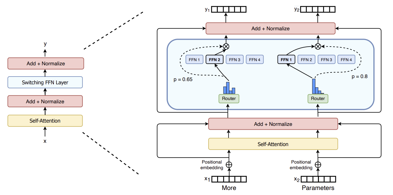
Mixture-of-Experts (MoE) is an old idea developed in 1989-1991 (e.g., see Robert A. Jacobs et al.). MoEs were later proved useful in deep learning, including for language models in 2017 by Noam Shazeer et al., then scaled to 1T parameter models in 2022 by William Fedus et al..

MoE from 2022 (Fedus et al.) with $N=4$. The figure shows only one expert (TopK=1) activated per token for clarity. Previously MoEs were often called "Switch Transformers".

As illustrated in the Figure above and formally defined below, MoE is a special neural network layer consisting of multiple expert networks ($E$)I drop the layer index for simplicity as the same equation is used for all layers (with trainable parameters in all layers being different unless shared). and a gating network ($g$) that selects which experts to use for $d$-dimensional input $\mathbf{x} \in \mathbb{R}^{n \times d}$ with $n$ tokens:

\[\mathbf{y}(\mathbf{x}) = \sum_{i=1}^{N} \underbrace{g(\mathbf{x})_i}_{\text{gate out}} \, \underbrace{E_i(\mathbf{x})}_{\text{expert out}},\]

where each $E_i$ has the same architecture as an FFNFFN stands for "feed-forward network", which is usually implemented as a simple MLP or a Gated Linear Unit (GLU) in Transformers. layer in Transformers. The gating network is typically implemented asThe order of the Softmax and TopKMask operations can vary in implementations.:

\[g(\mathbf{x}) = \text{TopKMask} \big( \text{Softmax} ( \underbrace{\mathbf{x} \, \mathbf{W}_g^T}_{\in \mathbb{R}^{n \times N}} ), \, \text{TopK} \big),\]

where $\mathbf{W}_g \in \mathbb{R}^{N \times d}$ are the gating weights, and TopKMask is an operation that retains only the TopK values per row (i.e. per token) and sets the rest to zero. Softmax is applied along each row to produce a probability distribution over the $N$ experts.

Expert Network Architecture

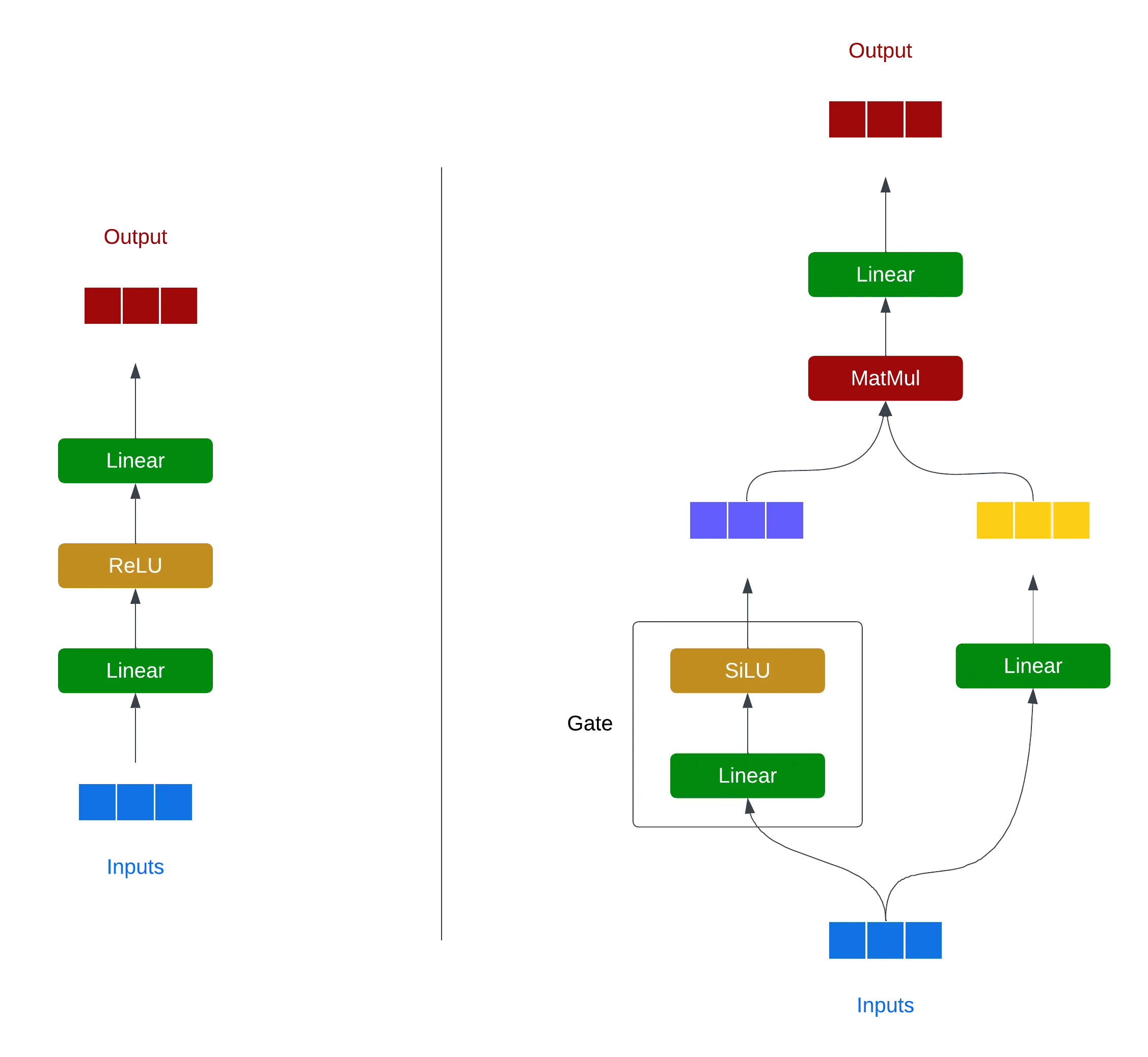
Simple FFN (left) vs GLU-based FFN used in modern MoEs (right). Source: medium.com/@achronus.

Each expert network $E_i$ is an FFN layer that processes the input $\mathbf{x}$ independently of other experts. Recent FFN layers in both original (non-MoE or “dense”) and MoE Transformers are based on Gated Linear Units (GLU) instead of simple MLPs:

\[E_i(\mathbf{x}) = \mathbf{W}_{i,\text{down}} \big( \text{act} (\mathbf{W}_{i,\text{gate}} \mathbf{x}) \odot (\mathbf{W}_{i,\text{up}} \mathbf{x}) \big), \; \text{for} \; i=1,...,N,\]

where act is SiLU/Swish or GELU, $\odot$ is element-wise multiplication; $\mathbf{W}_{i,\text{gate}}$ and $\mathbf{W}_{i,\text{up}}$
project $\mathbf{x}$ to a lower dimensional space (e.g., 2048 to 768 in Qwen3), $\mathbf{W}_{i,\text{down}}$ projects it back to the high dimensional space.

Key Concepts of MoE

Having defined an MoE layer above, let’s highlight the following key MoE concepts to better understand expert pruning and merging techniques:

MoE layers replace regular FFN (MLP) layers in Transformers (see the first Figure on the right). So for example in a Qwen3 model with 96 Transformer layers, there are 96 MoE layers (that are interleaved with self-attention layers within each Transformer layer).
Each MoE layer has $N$ experts (e.g., 128 in Qwen3 MoE models) with a Gated Linear Unit architecture described above. Having many FFNs massively increases the total number of parameters compared to non-MoE (dense) models (with $N=1$).
The gating network $g$ selects TopK experts (e.g., 8 in Qwen3 MoE models) for each input token based on its representation (row in $\mathbf{x}$) in the current Transformer layer. So for example, some experts in early layers learn to specialize on punctuation or number tokens, while in later layers they can specialize on more abstract concepts.
During inference, only the selected experts are used in the forward pass, making MoEs efficient (in terms of FLOPs) despite their large number of parameters. However, to make inference efficient in practice, expert weights need to be stored on GPUs to avoid data transfer overheads creating the memory demand.

Further technical details of MoE layers can be found in papers and a more animated and educational explanation in Maarten Grootendorst’s blog post.

Strengths of MoE

Although dense Transformers can learn from diverse data well, MoEs more explicitly promote distributed specialized knowledge. This is achieved by having multiple experts that can each specialize in different aspects of the data with the help of the gating mechanism that promotes sparsity.

It has been also shown that MoEs can scale well given a fixed FLOPs budget at inference (see the Figures below). Specifically, Tay et al. in 2022 showed that MoEs (or Switch Transformers back then) were one of the few architectures that demonstrated strong scaling trends in both upstream (pretraining) and downstream (fine-tuning) cases.

Upstream performance comparison (pretraining).

Downstream performance comparison (fine-tuned).

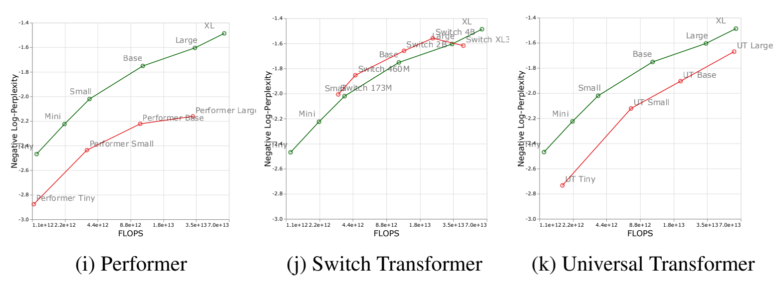
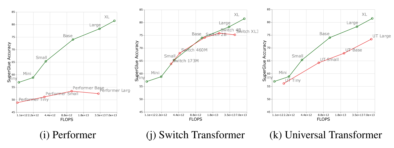
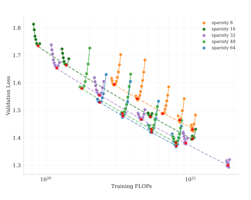
As figures above show, Switch Transformers still underperformed dense Transformers at the largest scale. However, the design choices and training of MoEs have improved since then (e.g., see), leading to even better scaling trends in recent MoE LLMs. Moreover, recently Kimi MoE LLMs demonstrated strong scaling trends with increasing MoE sparsity (see the Figure below). They define sparsity as the total number of experts ($N$) divided by TopK showing that for a fixed TopK increasing $N$ and, hence, sparsity consistently improves results.

Sparsity Scaling Law. Each point corresponds to training a model with a different number of experts and different hyperparameters (depth/width/number of steps/etc.). For example, for loss=1.5, sparsity=48 reduces FLOPs by 1.69$\times$, 1.39$\times$ and 1.15$\times$ compared to sparsity=8, 16 and 32, respectively.

These findings explain increasing the number of experts to 384 in Kimi K2 compared to 256 in DeepSeek and 128 in Qwen3 (more recent Qwen3-Next-80B-A3B also increased $N$ to 512). Even though the total number of parameter is soared to 1T, the inference remains efficient (with only TopK=8 experts activated). However, the memory demand to store all expert weights on GPUs becomes a bottleneck for deploying such large MoE LLMs.

Background: MoE Compression

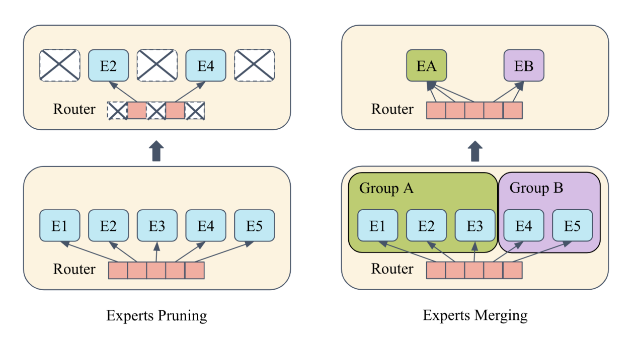
Let me briefly describe some key expert pruning and merging techniques below before presenting my approach and results. I follow an assumption standard in the MoE compression literature that there is a pretrained MoE model with $N$ experts per MoE layer and the goal is to reduce it to $k < N$ experts. I do not consider retraining/fine-tuning (or any further compression) after pruning/merging experts, which could be a complementary step.

Expert pruning vs merging (figure from the HC-SMoE paper).

Pruning Experts

Given hundreds of experts in each MoE layer, it is tempting to assume there is some redundancy in them and aim to reduce their number without sacrificing performance too much. One straightforward approach to do so is to prune some experts based on their activation frequencies. These frequencies are computed based on gate logits $g(\mathbf{x})$ by counting how often each of the $N$ experts is among TopK experts. For that purpose, we can forward pass some calibration data through the MoE layer and compute the activation frequencies (or saliency scores, $A$) for each expert. Given $A$, we keep only $ k < N $ experts with the highest scores.

The following is my pseudocode of computing activation frequencies $A$.

# Pseudocode for computing activation frequencies
N = 128  # number of experts
n = 1024  # number of tokens in calibration data
topk = 8  # TopK experts activated per token (based on the model configuration)

g = torch.randn(n, N)  # assume router logits for n tokens and N experts after some layer
g = torch.softmax(g, dim=-1) # apply softmax according to Equation above
topk_indices = torch.topk(g, k=topk, dim=-1).indices  # (n, topk)
# count how often each expert is selected
A = torch.zeros(N)
for i in range(N):
    A[i] = (topk_indices == i).sum().item()
# keep k < N experts with highest A

Recent Router-weighted Expert Activation Pruning (REAP) method significantly improves simple frequency counting. REAP defines $i$-th expert’s importance ($S_i$) based on the expert output’s norm weighted by the gate output:

\[S_i = \frac{1}{|\mathbf{x}^{(i)}|} \sum g_i(\mathbf{x}^{(i)}) \, || \, E_i(\mathbf{x}^{(i)}) || \text{ for } i=1,...,N,\]

where $\mathbf{x}^{(i)}$ is the subset of $\mathbf{x}$ corresponding to the tokens that activated expert $ i $. Compared to activation frequencies ($A$), scores $S$ measure more accurately the contribution of each expert to the final output of the MoE layer.

The following is my pseudocode of computing REAP scores based on the equation aboveMy implementation may differ from the official REAP code https://github.com/CerebrasResearch/reap. I implement a simple version aligned with the equation..

# Pseudocode for computing REAP scores
N = 128  # number of experts
n = 1024  # number of tokens in calibration data
topk = 8  # TopK experts activated per token (based on the model configuration)
d = 2048 # expert output dimension

expert_activations = torch.randn(N, n, d)  # assume expert outputs for n tokens and N experts after some layer

g = torch.randn(n, N)  # assume router logits for n tokens and N experts after some layer
g = torch.softmax(g, dim=-1) # apply softmax according to Equation above
topk_values, topk_indices = torch.topk(g, k=topk, dim=-1)  # (n, topk)

# compute REAP score for each expert
S = torch.zeros(N)
for i in range(N):
    # get tokens routed to expert i
    top_x, idx = torch.where(topk_indices == i)
    # top_x - indices of tokens activating expert i (values between 0 and n-1)
    # idx - indices of experts in topk (values between 0 and topk-1)
    if len(idx) == 0:
        continue  # no tokens activated expert i
    expert_state = expert_activations[i, top_x]  # (selected tokens, d)
    S[i] = (expert_state.norm(dim=-1) * topk_values[top_x, idx]).mean().item()
# keep k < N experts with highest S

Merging Experts

Compared to pruning experts, several works have explored merging them instead (e.g., ). The algorithms to merge experts typically have two steps applied to each MoE layer:

Grouping or clustering similar experts together based on some similarity metric.
Combining the weights of experts within each group to form a single expert.

Step 1 (grouping) is usually the key difference across the methods. For example, MC-SMoE finds $k$ cluster centroids first. To do so, the activation frequencies ($A$), defined above, are used as in pruning methods. However, in contrast to simply removing low-score experts as in pruning, MC-SMoE assigns them to the centroids based on the similarity of expert representations (e.g., expert weights or expert/gate logits given some calibration data). In HC-SMoE, the grouping step is based on hierarchical clustering of experts based on their outputs (also given some calibration data). HC-SMoE outperformed MC-SMoE, therefore I use HC-SMoE as a baseline in my experiments below.

Step 2 (combining) in both MC-SMoE and HC-SMoE involves weighted averaging of expert weights within each group, where the weighting coefficients are computed as in pruning methods (i.e., based on normalized activation frequencies $A$). In the next subsection, I describe an important nuance of this step.

Combining the Weights of Experts: Permutation Alignment

Computing the average of neural network weights can lead to poor results in certain casesIt is actually very surprising that averaging of weights can work at all in some cases, so papers like Model soups were very impactful.. Among such cases is when the networks are trained from different initializations and different data orderings/subsets. The difficulty of averaging weights in this case arises because of the different symmetries in neural network weights, primarily neuron permutation symmetry.

Neuron permutation symmetry states that the order of neurons in adjacent layers of a neural network layer can be randomly permuted without affecting the overall function of the network.

For example, in a 2 layer MLP, we can randomly permute rows of the first layer weights and permute in the same order the corresponding columns of the second layer weights without changing the function computed by the MLP.

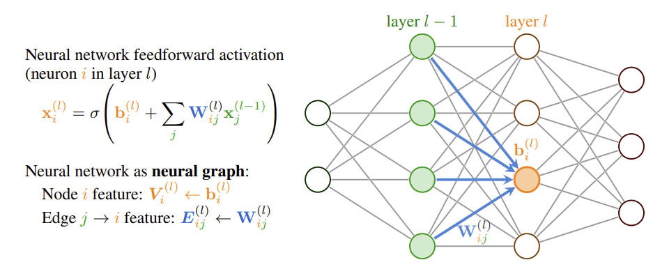
Neural network parameters can be represented as neural graphs to model neuron permutation symmetry.

Neuron permutation symmetry and other symmetries are studied in the Weight Space Learning (WSL) area of machine learning. One of the key findings in this area is that permutation alignment of the weights of one network w.r.t. another network prior to averaging can significantly improve the results. To model neuron permutation symmetry better, we proposed neural graphs and recently showed that we can train powerful graph neural networks based on neural graphs.

When training MoE LLMs, each expert network $E_i$ is initialized randomly and trained on different data subsets (because of the gating mechanism). To address the permutation issue, MC-SMoE and HC-SMoE align expert weights by either expert weights or hidden activations. This can be done, for example, using scipy.optimize.linear_sum_assignment function that implements the Hungarian algorithm to solve the assignment problem. I show a pseudocode for expert merging with improved permutation alignment in the next section.

REAM

My approach is based on REAP with merging instead of pruning, hence it is called Router-weighted Expert Activation Merging or REAM. It can also be seen as a modification of MC-SMoE with REAP scores and additional tricks as described below.

Algorithm

For each MoE layer with $N$ experts originally (and $k$ experts as a result):

Compute saliency scores $S$ for each expert as in REAP.
Pick $k$ experts with the highest $S$ and label them as cluster centroids similarly to MC-SMoE.
Group experts, but in contrast to MC-SMoE’s grouping, REAM uses pseudo-pruningThis is called pseudo-pruning, because most of the scores $S$ of the non-centroid experts will be low, so the weighted average (in step 5) will be dominated by the centroid expert.. The idea behind pseudo-pruning is to have a few big clusters and many singletons with unchanged weights. The grouping starts with the centroid having the highest $S$ and assigning $C$ most similar experts to it (that are not assigned yet). This step is repeated for all centroids until all $N$ experts are assigned ($C=16$ in my experiments).
The expert similarity metric, used in the previous step, is improved compared to prior work based on two key tricks. First, REAM uses an average of cosine similarity of expert outputs and cosine similarity of gate logits. Second, gated similarity is computed by multiplying expert outputs by gate logits motivated by the REAP equation.
Merge the weights in each group accounting for permutation alignment of weights based on both hidden activations and weights of $E$ as shown in the pseudocode below.
Use the merged MoE layer to compute the inputs for the next MoE layer. In contrast, previous works perform merging/pruning at each layer given the original inputs (i.e., computed using the original uncompressed model) to that layer. It means they can do pruning/merging in an arbitrary order of layers since the inputs/outputs are precomputed based on the original model. In REAM, the process is inherently sequentialTo implement sequential merging, calibration data has to be propagated through each MoE layer twice: first time to get necessary outputs to perform merging, second time to get the inputs for the next layer using the merged experts..

The highlighted steps are ablated in the Experiments section below.

The following pseudocode illustrates step 5 of merging a group of experts with permutation alignment based on both hidden activations and weights.

# Pseudo-code for merging a group of experts with logits+weights permutation alignment
G = 16 #  number of experts in a group (cluster) to be merged found in steps 3-4
d = 768 # bottleneck dimension in the expert network 
d_model = 2048 # model dimension

expert_hidden = torch.randn(G, d, n)  # hidden activations of G experts for n tokens in a MoE layer
expert_weights = torch.randn(G, d, d_model*3)   # concatenated expert weights in a group (3 weight matrices per expert)

# optional: perform dimensionality reduction and normalization steps on expert_weights

S = torch.rand(G)  # REAP scores for G experts in a group (from step 1)
S_norm = S / S.sum()  # normalized scores (sum=1)

avg_weights = S_norm[0] * expert_weights[0].clone()

# compute permutation cost matrices w.r.t. expert 0 
for i in range(1, G):
    cost1 = torch.cdist(expert_hidden[0], expert_hidden[i])    # (d, d)
    cost2 = torch.cdist(expert_weights[0], expert_weights[i])  # (d_model*3, d_model*3)
    row_ind, col_ind = scipy.optimize.linear_sum_assignment(cost1 + cost2)
    perm = col_ind  # permutation of expert i w.r.t. expert 0
    expert_weights[i] = expert_weights[i][perm]  # permute expert i hidden weights accordingly
    avg_weights += S_norm[i] * expert_weights[i]  # weighted average

# Result: G experts merged into one expert with avg_weights

Calibration Data

The design of calibration data is critical in expert pruning/merging methods. In expert merging and early pruning papers, the c4 dataset is often used. REAP uses c4 and/or evol-codealpaca depending on the downstream task. In my experiments, to make evaluation consistent while the model performant, a fixed mix of c4, math and coding data is used.

The calibration data consists of 2048 sequences from diverse sources. It is fixed in all my experiments for all the methods unless explicitly mentioned otherwise (like in ablations).

For math data, the AI-MO/NuminaMath-1.5 dataset is used, namely subsets ‘cn_k12’ and ‘olympiads’, with the idea to avoid the overlap with benchmark datasets. For coding data, bigcode/the-stack-smol is used. A different number of samples (sequences) and max tokens are used per dataset to balance their proportions as shown below.

Table 1. Calibration data used across all the experiments.

Domain	Dataset	Sequences	Max tokens	≈Total tokens	≈Proportion
General	allenai/c4/en	512	128	60k	8%
Math	AI-MO/NuminaMath-1.5 (cn_k12, olympiads)	1024	512	524k	68%
Coding	bigcode/the-stack-smol	512	512	190k	24%

Math and coding data are dominant as they are often shown important in adapting LLMs for reasoning and coding tasks. Also, math and coding benchmarks dominate the evaluation in practice. However, the exact proportion in REAM may be suboptimal and can be further explored in future work.

Gate Weight Adjustment

Finally, after experts are merged, the gate ($g$) weights have to be adjusted to account for the reduced number of experts. In expert merging implementations, merged experts are tied in memory instead of actually keeping only $k$ experts, while gate weights remain unchanged. This leads to gate logits corresponding to the experts within a merged group being summed during inference (see the REAP paper for additional analysis). In contrast, REAM follows REAP and simply removes the weights of the non-centroid experts from the gate weights.

Experiments

Experiments are run for three models: Qwen3-30B-A3B-Instruct-2507, Qwen3-235B-A22B-Instruct-2507 and Qwen3-Next-80B-A3B-Instruct. These are MoE LLMs with 30B, 235B and 80B parameters, respectively. Qwen3-30B-A3B and Qwen3-235B-A22B have $N$=128 experts and TopK=8The key differences between the two models are the number of Transformer layers (48 vs 94) and hidden size (2048 vs 4096).. Qwen3-Next-80B-A3B has $N$=512 experts and TopK=10. They are versatile models fine-tuned for instruction-following tasks heavily used in practice.

The experiments aim to reduce the number of experts by 25% (i.e., from 128 to 96 or from 512 to 384), while maintaining high performance across multiple benchmarks. The proposed REAM method is evaluated compared to the leading expert pruning method (REAP) and leading expert merging method (HC-SMoE).

🤗Qwen3 models compressed with HC-SMoE/REAP/REAM are released at huggingface-models. Details about the evaluation are provided at huggingface-details.

Benchmarks

Compressed models are evaluated on two sets of benchmarks: multi-choice question answering (MC) and long context reasoning tasks (GEN) tasks. The MC tasks are often evaluated by loglikelihood of the correct choice among multiple choices, so the model does not generate free-form text answers. In contrast, in long context reasoning tasks (GEN), the model need to generate free-form answers, which is often more challenging and useful in practice.

The MC set includes 8 tasks used in the HC-SMoE paper: Winogrande, ARC-C, ARC-E, BoolQ, HellaSwag, MMLU, OpenBookQA and RTE.

Table 2. GEN benchmarks used in the experiments.

Benchmark	Description	#Tasks
IFEval	General instruction-following	541
AIME25	Math reasoning, competitive high school level	30
GSM8K	Math reasoning, grade school level	1319
GPQA-Diamond	Scientific reasoning tasks in biology, physics and chemistry, PhD level	792
HumanEval (instruct)	Python code generation tasks	164
LiveCodeBench v6	More challenging code generation tasks	1055

Qwen3-30B-A3B

Qwen3-30B-A3B-Instruct-2507 was used to tune the REAM hyperparameters (like calibration data mix, number of experts per group $C$, etc.). Also, several ablations of REAM are performed using this model to highlight the importance of REAM components. The results are shown in the Figure below with the average scores across MC ($x$ axis) and GEN tasks ($y$ axis).

{
  "data": [
    {
      "name": "Original",
      "type": "scatter",
      "mode": "markers",
      "x": [69.7],
      "y": [70.9],
      "marker": { "size": 12, "symbol": "circle" }
    },
    {
      "name": "HC-SMoE (c4)",
      "type": "scatter",
      "mode": "markers",
      "x": [63.3],
      "y": [65.2],
      "marker": { "size": 12, "symbol": "square" }
    },
    {
      "name": "HC-SMoE",
      "type": "scatter",
      "mode": "markers",
      "x": [64.9],
      "y": [66.3],
      "marker": { "size": 12, "symbol": "diamond" }
    },
    {
      "name": "REAP",
      "type": "scatter",
      "mode": "markers",
      "x": [65.0],
      "y": [64.2],
      "marker": { "size": 12, "symbol": "cross" }
    },
    {
      "name": "REAM",
      "type": "scatter",
      "mode": "markers",
      "x": [65.8],
      "y": [67.7],
      "marker": { "size": 15, "symbol": "star" }
    },
    {
      "name": "REAM (c4)",
      "type": "scatter",
      "mode": "markers",
      "x": [69.3],
      "y": [35.3],
      "marker": { "size": 10, "symbol": "x" }
    },
    {
      "name": "REAM (no REAP)",
      "type": "scatter",
      "mode": "markers",
      "x": [52.3],
      "y": [64.1],
      "marker": { "size": 10, "symbol": "triangle-up" }
    },
    {
      "name": "REAM (no gated sim)",
      "type": "scatter",
      "mode": "markers",
      "x": [64.6],
      "y": [51.3],
      "marker": { "size": 10, "symbol": "triangle-down" }
    },
    {
      "name": "REAM (no pseudo-pruning)",
      "type": "scatter",
      "mode": "markers",
      "x": [63.5],
      "y": [61.3],
      "marker": { "size": 10, "symbol": "triangle-right" }
    },
    {
      "name": "REAM (no seq)",
      "type": "scatter",
      "mode": "markers",
      "x": [65.5],
      "y": [66.0],
      "marker": { "size": 10, "symbol": "triangle-left" }
    }    
  ],
  "layout": {
    "title": "Pareto Tradeoff Between MC and Generation",
    "xaxis": {
      "title": { "text": "MC tasks score (%)" },
      "range": [45, 77]
    },
    "yaxis": {
      "title": { "text": "GEN tasks score (%)" },
      "range": [34, 77]
    },
    "legend": {
      "orientation": "v"
    }
  }
}

REAM obtains 65.8% and 67.7% average scores on MC and GEN tasks, respectively, while the original model achieves 69.7% and 70.9%. HC-SMoE and REAP achieve 64.8%/66.3% and 65.2%/64.1%, respectively, with REAP being better on MC tasks and HC-SMoE being better on GEN tasks. The proposed REAM method outperforms both of them.

The ablations highlight the importance of REAM components. Notably, using only c4 as calibration data significantly degrades GEN tasks performance, however it makes MC tasks performance close to the original model. On the contrary, HC-SMoE is not as sensitive to the calibration data choiceThis result confirms the stability of HC-SMoE regardless data as shown in their paper..

Another important component of REAM is using REAP scores for selecting centroids. When simple frequency-based scores are used instead, the performance (especially MC) drops significantly. Using proposed gated similarity, pseudo-pruning and sequential merging also improve the results with gated similarity being the most important among them.

Interestingly, the results reveal an inherent tradeoff between MC and GEN tasks performance when compressing MoE LLMs. Achieving Pareto optimal results seems challenging, however REAM shows promising results in this direction.

Detailed results per task are shown below.

Table 3. MC results for Qwen3-30B-A3B-Instruct-2507.

Model	N	Winogrande	ARC-C	ARC-E	BoolQ	HellaSwag	MMLU	OBQA	RTE	AVG
Original	128	73.2	60.7	85.1	88.7	61.2	80.1	32.4	76.5	69.7
REAM	96	71.8	51.9	79.1	88.5	57.6	70.1	30.0	77.6	65.8

Table 4. GEN results for Qwen3-30B-A3B-Instruct-2507.

Model	N	IFEval	AIME25	GSM8K	GPQA-D	HumanEval	LiveCodeBench	AVG
Original	128	90.4	56.7	89.3	47.0	93.3	48.6	70.9
REAM	96	89.2	66.7	88.1	38.9	86.6	36.9	67.7

Qwen3-235B-A22B

Results on Qwen3-235B-A22B-Instruct-2507 are obtained by running REAM and baselines with the same hyperparameters and calibration data as for Qwen3-30B-A3B-Instruct-2507. So no tuning specific to this model is performed.

Evaluation on a model of this size is very challenging and computationally expensive. Specifically, 8xH100 GPUs were required to fit the model in memory and perform evaluationIn comparison, for Qwen3-30B, 1-4 GPUs were sufficient depending on the task.. Each task took from a few minutes to 1-2 hours to evaluate. So evaluation is costly, especially in academic settings. The results are shown in the Table below.

Table 5. GEN results for Qwen3-235B-A22B-Instruct-2507.

Model	N	IFEval	AIME25	GSM8K	GPQA-D	HumanEval	LiveCodeBench	AVG
Original	128	93.3	66.7	89.4	48.5	95.1	46.4	73.2
HC-SMoE	96	89.6	63.3	87.5	39.9	86.0	40.0	67.7
REAP	96	92.0	63.3	88.8	46.0	94.5	53.1	72.9
REAM	96	90.4	63.3	88.2	44.4	94.5	49.5	71.7

On Qwen3-235B-A22B-Instruct-2507, REAP slightly outperforms REAM on 4 out of 6 GEN tasks and on average. However, both achieve the results surprisingly close to the original model (even outperforming the original model on some tasks!). HC-SMoE lags behind both methods significantly, which is different from the results on Qwen3-30B-A3B-Instruct-2507. It is possible that hyperparameters of REAM (as well as the baselines) are suboptimal for this model, so further tuning may improve the results.

Qwen3-Next-80B-A3B

Qwen3-Next-80B-A3B-Instruct-2507 is a newer MoE model with a similar architecture as Qwen3-30B-A3B, but with 512 experts and TopK=10 instead of 128 and TopK=8, respectively. Even though the total number of experts is increased 4x, the number of activated parameters is mainly affected by TopK. And although TopK is also increased in this model, to keep the number of activated parameters around 3B, the bottleneck dimension in each expert is reduced from 768 to 512. The results of compressing this model from 512 to 384 experts are shown below. Other than the number of experts and TopK, the same hyperparameters and calibration data as for Qwen3-30B-A3B-Instruct-2507 are used in all methods.

Table 6. GEN results for Qwen3-Next-80B-A3B-Instruct-2507.

Model	N	IFEval	AIME25	GSM8K	GPQA-D	HumanEval	LiveCodeBench	AVG
Original	512	93.4	80.0	78.6	47.0	95.1	43.2	72.9
REAP	384	91.0	66.7	78.8	37.9	91.5	45.0	68.5
REAM	384	91.5	73.3	78.4	36.9	92.7	42.9	69.3

On Qwen3-Next-80B-A3B-Instruct-2507, REAM outperforms REAP on 3 out of 6 GEN tasks and on average. HC-SMoE was not evaluated on this model, since it underperformed in previous experiments. Notably, the original Qwen3-Next model has almost the same GEN performance as its previous much larger (Qwen3-235B-A22B) variant (see Table 5 above), while having only 3B activated parameters instead of 22B. This further confirms the effectiveness of increasing MoE sparsity.

Conclusion

Merging vs Pruning. REAM shows promising results by reducing the memory requirement by around 25% while maintaining high performance across multiple benchmarks. There is still a room for improvement, especially in merging methods to better combine the weights of multiple experts. So it is possible that pruning methods (REAP) remain strong because the merging methods are still quite suboptimal. Improving merging methods may allow for further reducing the number of experts (e.g., by 50%), while maintaining high performance.

MC vs GEN Tradeoff. The tradeoff between MC and GEN tasks performance is surprising, since MC tasks are assumed to be easier than GEN tasks. So I mistakenly expected that improving GEN tasks performance would also lead to better MC results.

High Engineering and Computation Barrier. Another observation is that evaluation of LLMs is way more challenging than expected, in some cases taking more time to set up properly than doing research. Besides the high engineering and computation barrier, some benchmarks such as AIME25 are quite noisy because of the small number of samples (30 questions). So evaluation should be done on more diverse and larger benchmarks, further increasing the engineering and computational cost.

Weight Space Learning. Finally, relying on calibration data is generally undesirable, because the results may be sensitive to the data choice. However, only using the weights of experts have led to poor results in my experiments and in ablation studies in the literature. Future work may explore how to use Weight Space Learning (WSL) and specifically methods based on neural graphs to better perform merging without relying on calibration data.

Citation

@misc{knyazev2026compressing,
  title={REAM: Compressing Mixture-of-Experts LLMs},
  author={Boris Knyazev},
  year={2026},
  url={https://bknyaz.github.io/2026/01/15/moe/}
}

Use of LLMs: LLMs were used to slightly improve the writing and formatting of this blog post.

Enjoy Reading This Article?

Here are some more articles you might like to read next:

Tutorial on Graph Neural Networks for Computer Vision and Beyond (Part 1)

Anisotropic, Dynamic, Spectral and Multiscale Filters Defined on Graphs

Spectral Graph Convolution Explained and Implemented Step By Step

Can we do better than Convolutional Neural Networks?

Training LLMs Faster by Learning Neuron Interaction