NiNo: Learning to Accelerate Training of Neural Networks

Explaining our ICLR 2025 paper and visualizing neuron permutation symmetry.

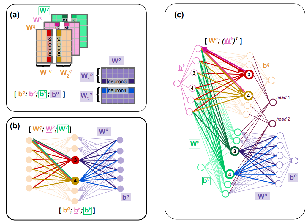
Training large neural networks is famously slow and expensive. In our paper, Accelerating Training with Neuron Interaction and Nowcasting Networks, presented at ICLR 2025 in Singapore, we introduced a new way to speed things up. We treat a neural network as a graph of interacting neurons, or neural graph, and train a graph neural network (GNN) to predict how the parameters of the network will evolve during training.

From Adam to NiNo

Due to massive training costs, recent years have seen a surge of faster adaptive optimizers: Shampoo, SOAP, Muon, and others. Each improves on Adam by smarter scaling and/or orthogonalization of parameter updates for a given weight matrix, often inspired by second-order methods or preconditioning. But they work at the level of parameters or layers, not the network as a whole. Moreover, they do not learn from the previous optimization runs, i.e., the optimization algorithms are based on manually-designed gradient-descent rules. Our method, NiNo (Neuron Interaction and Nowcasting), is different. Motivated by Kofinas et al., we model neurons as nodes and weights as edges, and use a graph neural network (GNN) to predict how weights will evolve. This lets us “nowcast” future parameters and reduce the number of steps required to reach the same performance metric.

NiNo is a GNN-based model that takes a history of past parameter values along the optimization trajectory (obtained with Adam or another optimizer) and makes a jump by predicting future parameter values. After making the prediction, optimization is continued with Adam, then followed by NiNo’s another prediction and so on.

This periodic nowcasting idea is borrowed from Weight Nowcaster Network (WNN) that revealed predictable patterns in optimization trajectories, but neural graphs synergized with GNNs make it work really well. To give some context in terms of optimization runs, below is Figure 1 reproduced from the NiNo paper.

{
  "data": [
    {
      "type": "scatter",
      "name": "Adam",
      "x": [
        645.4,
        1098.0,
        1559.6,
        2021.3,
        2482.9,
        2944.5,
        3406.2,
        3472.6,
        3867.8,
        4329.4,
        4791.1,
        5252.7,
        5714.3,
        6176.0,
        6637.6,
        6769.6,
        7099.3,
        7560.9,
        8022.5,
        8484.2,
        8945.8,
        9407.4,
        9869.1,
        10066.6,
        10330.7,
        10792.3,
        11254.0,
        11715.6,
        12177.2,
        12638.9,
        13100.5,
        13363.6
      ],
      "y": [
        1290.42,
        654.89,
        491.01,
        415.95,
        367.21,
        333.12,
        306.04,
        302.24,
        282.43,
        264.16,
        246.73,
        233.03,
        221.53,
        211.24,
        202.02,
        199.9,
        194.86,
        187.62,
        181.82,
        176.28,
        171.77,
        167.21,
        163.92,
        162.06,
        160.25,
        157.63,
        153.97,
        151.23,
        149.08,
        146.99,
        144.91,
        144.02
      ],
      "mode": "lines",
      "line": {
        "color": "#1f77b4",
        "width": 2.5
      }
    },
    {
      "type": "scatter",
      "name": "WNN (Jang et al., 2023)",
      "x": [
        654.8,
        1098.0,
        1559.6,
        2021.3,
        2482.9,
        2944.5,
        3406.2,
        3472.6,
        3867.8,
        4329.4,
        4791.1,
        5252.7,
        5714.3,
        6176.0,
        6637.6,
        6769.6,
        7099.3,
        7560.9,
        8022.5,
        8484.2,
        8945.8,
        9407.4,
        9869.1,
        10066.6,
        10330.7,
        10792.3,
        11254.0,
        11715.6,
        12177.2,
        12638.9,
        13100.5,
        13363.6
      ],
      "y": [
        1290.42,
        653.73,
        444.74,
        387.85,
        326.93,
        303.61,
        266.84,
        264.77,
        251.27,
        227.12,
        216.34,
        199.39,
        192.44,
        180.71,
        175.41,
        170.13,
        167.42,
        163.54,
        157.7,
        154.93,
        150.43,
        148.24,
        144.45,
        143.78,
        143.02,
        140.42,
        138.9,
        136.51,
        135.4,
        133.53,
        132.68,
        131.58
      ],
      "mode": "lines",
      "line": {
        "color": "#2ca02c",
        "width": 3,
        "dash": "dash"
      }
    },
    {
      "type": "scatter",
      "name": "NiNo (ours)",
      "x": [
        648.7,
        1098.0,
        1559.6,
        2021.3,
        2482.9,
        2944.5,
        3406.2,
        3472.6,
        3867.8,
        4329.4,
        4791.1,
        5252.7,
        5714.3,
        6176.0,
        6637.6,
        6769.6,
        7099.3,
        7560.9,
        8022.5,
        8484.2,
        8945.8,
        9407.4,
        9869.1,
        10066.6,
        10330.7,
        10792.3,
        11254.0,
        11715.6,
        12177.2,
        12638.9,
        13100.5,
        13363.6
      ],
      "y": [
        1290.42,
        652.54,
        425.26,
        371.58,
        294.78,
        271.73,
        231.12,
        228.8,
        217.43,
        193.29,
        184.29,
        169.48,
        163.7,
        154.62,
        150.46,
        149.22,
        144.61,
        141.77,
        138.42,
        136.37,
        134.1,
        132.88,
        131.09,
        130.71,
        130.05,
        128.99,
        128.08,
        127.1,
        126.53,
        125.55,
        124.76,
        124.48
      ],
      "mode": "lines",
      "line": {
        "color": "#D44841",
        "width": 5
      }
    },
    {
      "type": "scatter",
      "name": "target perplexity",
      "x": [
        636.4,
        13363.6
      ],
      "y": [
        147.0,
        147.0
      ],
      "mode": "lines",
      "line": {
        "color": "#7f7f7f",
        "width": 2,
        "dash": "dot"
      }
    }
  ],
  "layout": {
    "title": {
      "text": "NiNo achieves ~2× speedup compared to Adam.",
      "font": {
        "size": 20
      }
    },
    "xaxis": {
      "title": "training iteration",
      "range": [
        0,
        14000
      ],
      "tickvals": [
        0,
        2000,
        4000,
        6000,
        8000,
        10000,
        12000,
        14000
      ]
    },
    "yaxis": {
      "title": "validation perplexity",
      "type": "log",
      "range": [
        2,
        3
      ],
      "tickvals": [
        100,
        200,
        300,
        400,
        600,
        1000
      ],
      "ticktext": [
        "10\u00b2",
        "2\u00d710\u00b2",
        "3\u00d710\u00b2",
        "4\u00d710\u00b2",
        "6\u00d710\u00b2",
        "10\u00b3"
      ]
    },
    "legend": {
      "x": 1.0,
      "y": 1.0,
      "xanchor": "right",
      "yanchor": "top"
    },
    "margin": {
      "l": 70,
      "r": 20,
      "t": 60,
      "b": 60
    },
    "annotations": [
      {
        "x": 300,
        "xref": "x",
        "y": 0.60,
        "yref": "paper",
        "text": "Nowcast",
        "showarrow": false,
        "textangle": -45,
        "font": {
          "size": 10
        },
        "xanchor": "left",
        "yanchor": "bottom"
      },
      {
        "x": 1300,
        "xref": "x",
        "y": 0.40,
        "yref": "paper",
        "text": "Nowcast",
        "showarrow": false,
        "textangle": -45,
        "font": {
          "size": 10
        },
        "xanchor": "left",
        "yanchor": "bottom"
      },
      {
        "x": 10300,
        "xref": "x",
        "y": -0.03,
        "yref": "paper",
        "text": "Nowcast",
        "showarrow": false,
        "textangle": -45,
        "font": {
          "size": 10
        },
        "xanchor": "left",
        "yanchor": "bottom"
      }
    ]
  }
}

The figure shows the results of Adam without and with nowcasting using our NiNo. “Nowcast” steps are shown at step 1000, 2000 and 11,000 for visualization purposes, but this step is applied every 1000 steps in our experiments. Note the ~2× reduction of the number of steps required by NiNo to achieve the same validation perplexity as by Adam. The optimization task in this example is autoregressive next-token prediction on the WikiText103 dataset that NiNo has not seen during its training.

NiNo Details

As NiNo is a neural network (namely, a GNN), it needs to be trained first before we can use it to speed up optimization. To do so, we collected and publicly released a 🤗dataset of checkpoints with optimization trajectories on 2 vision and 2 language tasks. Even though collecting these checkpoints and training NiNo is computationally expensive, this one-time cost is amortized, meaning the same trained NiNo can potentially be used across many tasks, ultimately reducing total training cost.

Neuron Permutation Symmetry

Developing a strong parameter nowcasting model requires many specific design choices and, perhaps most critically, accurate modeling of neuron permutation symmetryModeling neuron permutation symmetry imposes a strong inductive bias similarly to using convolution for images. So our model can be used in more diverse tasks and should be able to learn parameter prediction rules that generalize better with fewer samples compared to models that do not explicitly take this symmetry into account.. Neuron permutation symmetry states that the order of neurons in adjacent layers of a neural network can be permuted in certain ways without affecting the overall function of the network. To better understand this symmetry, let me introduce a simple example based on a two layer neural network with weights $\mathbf{W}_1$, $\mathbf{W}_2$ and an element-wise activation function σ. Given input $\mathbf{x}$, the output of such a network can be expressed as:

\[f(\mathbf{x}) = \mathbf{W}_2 \ \sigma(\mathbf{W}_1 \ \mathbf{x}).\]

We can permute the neurons in the hidden layer by applying a permutation matrix $\mathbf{P}$ to the weights in layer 1 (permuting rows) and the inverse permutation to the weights in layer 2 (permuting columns), resulting in:

\[f(\mathbf{x}) = (\mathbf{W}_2 \ P^{-1}) \ \sigma(P \ \mathbf{W}_1 \ \mathbf{x}).\]

Given the orthogonality property of permutation matrices, $\mathbf{P}^{-1} = \mathbf{P}^T$, and that the activation function σ is element-wise, we can see that the output of the network remains unchanged:

\[f(\mathbf{x}) = \mathbf{W}_2 \ \mathbf{P}^{-1} \ \sigma ( \mathbf{P} \ \mathbf{W}_1 \ \mathbf{x}) = \mathbf{W}_2 \ \mathbf{P}^{-1} \mathbf{P} \ \sigma (\mathbf{W}_1 \ \mathbf{x}) = \mathbf{W}_2 \ \sigma(\mathbf{W}_1 \ \mathbf{x}).\]

Let me now visualize this symmetry using a simple demo, where the output is dynamically computed given the current order of neurons for some fixed input. You can click the “Swap Random Pair” button to randomly swap two (just for simplicity) hidden neurons and see how the network diagram and weight matrices change, while the computed output should (hopefully!) remain the same. You can also toggle the “Correct Permutation” option off to turn off the permutation of the weights in the second layer, in which case the output changes. You can reset the demo to the original state by clicking the “Reset” button.

Input x:

Hidden h:

Output y:

💡 Watch how swapping two hidden neurons changes the network diagram and weight matrices, but the output stays the same!

Neuron Permutation Symmetry in Transformers

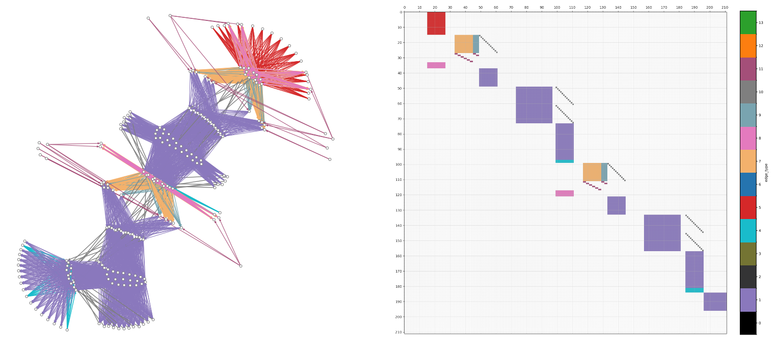
To make NiNo work well for LLMs and Transformers in general, it was critical to carefully construct the neural graph for multi-head self-attention, making it stand out compared to WNN (which ignores the neural network structure). This is a tricky part as the illustration below shows, but we implemented it for many different Transformer layers.

Constructing neural graphs for a MSA layer (see the details in our paper and code).

Visualizing the permutation symmetry in Transformers using a demo is also possible, but I leave it for future work (or please submit a PR to this blog post).

Results that Stand Out

NiNo achieves roughly a 2× speedup compared to Adam, which is rarely achieved by manually designed optimizers in practiceWhich are considered remarkable if a 1.2–1.3× speedup is achieved..
NiNo speeds up optimization across 9 vision and language tasks that we systematically evaluated, achieving the same validation performance (accuracy or perplexity) as Adam in about half the steps on average across these tasks (see Table 2 in the paper).
NiNo continues to speed up training for larger models beyond our main 9 tasks that are much larger than the models in the training checkpoints used to train NiNo (see Table 4 in the paper).

In addition, as shown below, applying NiNo is straightforward:

import torch
import torch.nn.functional as F
from transformers import AutoModelForCausalLM
from optim import NiNo

model = AutoModelForCausalLM.from_config(...)  # some model

# NiNo is implemented as a wrapper around the base optimizer
# any optimizer other than Adam should also be possible to use with NiNo
opt = NiNo(base_opt=torch.optim.AdamW(model.parameters(), 
           lr=1e-3, 
           weight_decay=1e-2),
           ckpt='checkpoints/nino.pt',
           subgraph=False, # can be set to True for larger models (see Llama 3.2 example below)
           edge_sample_ratio=0,  # can be set to a small positive number for larger models (see Llama 3.2 example below)
           model=model,
           period=1000,
           max_train_steps=10000)
for step in range(10000):
    if opt.need_grads:  # True/False based on the step number and period
        opt.zero_grad()  # zero out gradients
        data, targets = ...  # get some batch of data
        # base optimizer step (majority of the time)
        outputs = model(data)  # forward pass
        loss = F.cross_entropy(outputs, targets)  # compute some loss
        loss.backward()  # only compute gradients for the base optimizer            
    opt.step()  # base_opt step or nowcast params every 1000 steps using NiNo    

Learning to Optimize, Revisited

Our work connects to the broader “learning to optimize” literature, such as VeLO. Unlike many learned optimizers that struggle with cost, stability or show only a ~1.2–1.3× speedupWhile a ~1.2–1.3× speedup is remarkable, in practice it usually does not justify the immense amount of extra work (e.g. efficient distributed implementation, tuning, potential instabilities especially in mixed/low-bit precision, investigating unexpected side effects like overfitting or poor generalization) that is required for actual large-scale usefulness., NiNo is conceptually lightweight and stable, because it is only applied every 1,000 steps (by default), while for all the other steps any base optimizer, such as Adam, can be applied to allow for stable convergence. At the same time, recent learned optimizers such as our recent Celo and μLO that will be presented at ICLR 2026, make a significant step in improving learned optimizersIn particular, Celo and μLO make learned optimizers more cost-effective and stable (i.e. without big loss spikes) to train and use..

Neural graph of a Llama-3 based architecture (graph and adjacency matrix are visualized, see the paper for details). In the code, we also support many other architectures, including Qwen3 and vision models like ViT.

Conclusion

Even though NiNo shows great speedups, it requires further work, for example:

Making NiNo’s step more scalable (especially memory-efficient) to larger models - currently the message passing step in its GNN is a bottleneck;
Improving speedups on larger tasks - for tasks with >1B parameter models we currently observe no speedup;
Adding automatic ways to construct neural graphs and verify their correctness;
Combining NiNo with learned optimizers to get the merits of both;
Showing theoretical guarantees for convergence.

We have open-sourced our code and pretrained NiNo checkpoints at github.com/SamsungSAILMontreal/nino under MIT License and welcome contributions.

License

Diagrams and text are licensed under Creative Commons Attribution CC-BY 4.0, unless noted otherwise.

Citation

@inproceedings{knyazev2024accelerating,
  title={Accelerating Training with Neuron Interaction and Nowcasting Networks}, 
  author={Boris Knyazev and Abhinav Moudgil and Guillaume Lajoie and Eugene Belilovsky and Simon Lacoste-Julien},  
  booktitle={International Conference on Learning Representations},
  year={2025},
}

Enjoy Reading This Article?

Here are some more articles you might like to read next:

Tutorial on Graph Neural Networks for Computer Vision and Beyond (Part 1)

Anisotropic, Dynamic, Spectral and Multiscale Filters Defined on Graphs

Spectral Graph Convolution Explained and Implemented Step By Step

Can we do better than Convolutional Neural Networks?

MetaMerge: Model Merging with Meta Networks