The British Machine Vision Conference (BMVC), finished about two weeks ago in Cardiff, UK, is one of the top conferences in computer vision & pattern recognition with a competitive acceptance rate of 28%. Compared to others, it’s a small event, so you have plenty of time to walk around posters and talk to presenters one-on-one, which I found really nice.
Paper decisions were released yesterday. Congratulations to all of you! In total, we received 1008 submissions, of which 815 were valid. Of these, a total of 231 papers were accepted (38 as Oral Presentations, 193 as Poster Presentations). This amounts to a 28% acceptance rate.
I presented a poster on Image Classification with Hierarchical Multigraph Networks on which I mainly worked during my internship at SRI International under the supervision of Xiao Lin, Mohamed Amer (homepage) and my PhD advisor Graham Taylor.
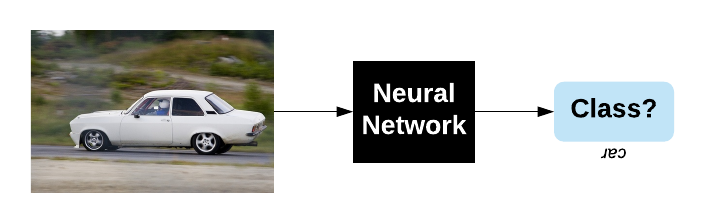
In the paper, we basically try to answer the question “Can we do better than Convolutional Neural Networks?”. Here I discuss this question and support my arguments by results. I also walk you through the forward pass of the whole pipeline for a single image from PASCAL VOC 2012 using PyTorch.
The complete code for this post is in my notebook on Github. It should be easy to adapt it for training and validating on the whole PASCAL dataset.
So, why do we want to do better than ConvNets? Haven’t they outperformed humans in many tasks?
For example, you could say that image classification is a solved task. Well, in terms of ImageNet, yes. But despite great contribution of ImageNet, it is a weird task. Why would you want to discriminate between hundreds of dog breeds? So, in result we have models succeeding in that, but failing to discriminate between slightly rotated dogs and cats. Fortunately, we now have ImageNet-C and other similar benchmarks showing that we are nowhere close to solving it.
Another open problem arising in related tasks, like object detection, is training on really large images (e.g., 4000×3000), which is addressed, for example, by Katharopoulos & Fleuret (ICML, 2019) and Ramapuram et al. (BMVC, 2019). Thanks to the latter I now know that if the background of a poster is black, then it’s likely from Apple. I should reserve some color too!
So, maybe we need something different than a Convolutional Neural Network? Instead of constantly patching its bugs, maybe we should use a model that has nicer properties from the beginning?
We argue that such a model can be a Graph Neural Network (GNN) — a neural network that can learn from graph-structured data. GNNs have some appealing properties. For example, compared to ConvNets, GNNs are inherently rotation and translation invariant, because there is simply no notion of rotation or translation in graphs, i.e. there is no left and right, there are only “neighbors” in some sense (Khasanova & Frossard, ICML, 2017). So, the problem of making a ConvNet generalize better to different rotations, that people have been trying to solve for years, is solved automatically with GNNs!
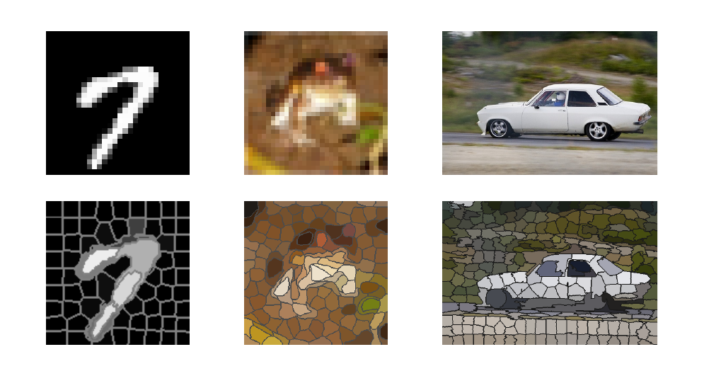
Regarding learning from large images, how about extracting superpixels from images and feeding a much lower dimensional input to a GNN instead of feeding a downsampled (e.g. 224×224) image to a ConvNet? Superpixels seem to be a much better way to downsample an image compared to, say, bilinear interpolation, because they often preserve a lot of semantics by keeping the boundaries between objects. With a ConvNet we cannot directly learn from this kind of an input, however, there are some nice works proposing to leverage them (Kwak et al., AAAI, 2017).
So, a GNN sounds wonderful! Let’s see how it performs in practice.
Oh no! Our baseline GNN based on (Kipf & Welling, ICLR, 2017) achieves merely 19.2% (mean average precision or mAP) on PASCAL, compared to 32.7% of a ConvNet with the same number of layers and filters in each layer.
We propose several improvements that eventually beat the ConvNet!
In ConvNets, the hierarchical structure of images is implicitly modeled by pooling layers. In GNNs, you can achieve this in at least two ways. First, you can use pooling similar to ConvNets, but for graphs, defining a fast and good pooling method is really challenging. Instead, we can compute superpixels at multiple scales and pool superpixels by their correspondence to a larger parent superpixel. However, for some reasons this kind of pooling didn’t work well in our case (I still think it should work well). So, instead we model a hierarchy at the input level. In particular, we combine superpixels of all scales into a single set and compute hierarchical relations based on intersection over union (IoU), commonly used in semantic segmentation.
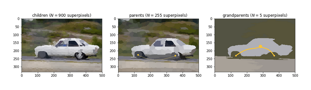
Based on that principle, I build the hierarchical graph in the code below. I also build a multiscale version of the spatial graph, but it encodes only spatial relationships, while IoU should better encode hierarchical ones. For example, using IoU we can create shortcuts between remote child nodes, i.e. connect two small superpixels (e.g., wheels) that are far away spatially, but belong to the same parent node (e.g., a car) as shown on the image above.
And indeed, the hierarchical graph boosts mAP to 31.7%, making it just 1% lower than a ConvNet while having 4 times fewer trainable parameters! If we use only the spatial multiscale graph, the results are much worse as explored in the paper.
Great! What else can we do to further improve results?
So far, if we visualize our filters, they will look very primitive (as Gaussians). See my tutorial on GNNs for more details. We want to learn some edge detectors similar to ConvNets, because they work so well. But it turned out to be very challenging to learn them with GNNs. To do that, we basically need to generate edges between superpixels depending on the difference between coordinates. By doing so, we will endow our GNN with the ability to understand the coordinate system (rotation, translation). We will use a 2 layer neural network defined in PyTorch like this:
pred_edge = nn.Sequential(nn.Linear(2, 32),
                          nn.ReLU(True),
                          nn.Linear(32, L))
where L is the number of predicted edges or the number of filters, such as 4 in the visualization below.
We restrict the filter to learn edges only based on the absolute difference between coordinates, |(x₁,y₁) - (x₂,y₂)|, instead of raw values, so that the filters become symmetric. This limits the capacity of filters, but it is still much better than a simple Gaussian filter used by our baseline GCN.
In my Jupyter notebook, I created a class LearnableGraph that implements the logic to predict edges given node coordinates (or any other features) and the spatial graph. The latter is used to define a small local neighborhood around each node to avoid predicting edges for all possible node pairs, because it’s expensive and doesn’t make much sense to connect very remote superpixels.
Below, I visualize the trained pred_edge function. To do that, I assume that the current node with index 1, where we apply the convolution, is in the center of a coordinate system, (x₁,y₁)=0. Then I simply sample coordinates of other nodes, (x₂,y₂), and feed them to pred_edge. The color shows the strength of an edge depending on the distance from a center node.

The learned graph is also very powerful, but at a larger computational cost, which is negligible if we generate a very sparse graph. The result of 32.3% is just 0.4% lower than a ConvNet and can be easily improved if we generate more filters!
We now have three graphs: spatial, hierarchical and learned. A single graph convolutional layer with the spatial or hierarchical graph permits feature propagation only within the “first neighbors”. Neighbors are soft in our case, since we use a Gaussian to define the spatial graph and IoU for the hierarchical one. Defferrard et al. (NIPS, 2016) proposed a multiscale (multihop) graph convolution, which aggregates features within a K-hop neighborhood and approximates spectral graph convolution. See my other post for an extensive explanation of this method. For our spatial graph, it essentially corresponds to using multiple Gaussians of different width. For the hierarchical graph, this way we can create K-hop shortcuts between remote child nodes. For the learned graph, this method will create multiple scales of the learned filters visualized above.
Using multiscale graph convolution, implemented in my GraphLayerMultiscale class, turned out to be extremely important allowing us to outperform the baseline ConvNet by 0.3%!
So far, to learn from our three graphs, we have used a standard concatenation method. This method, however, has a couple of problems. First, the number of trainable parameters of such a fusion operator is linear w.r.t. the input and output feature dimensionalities, scale (K) and number of relation types, so it can really grow fast if we increase two or more of these parameters at once. Second, the relation types we try to fuse can have very different natures and occupy very different subspaces of a manifold. To solve both problems at the same time, we propose learnable projections similar to (Knyazev et al., NeurIPS-W, 2018). This way we decouple the linear dependency reducing the number of parameters by a factor of 2–3 compared to concatenation. In addition, learnable projections transform multirelational features so that they should occupy nearby subspaces of the manifold, facilitating the propagation of information from one relationship to another.
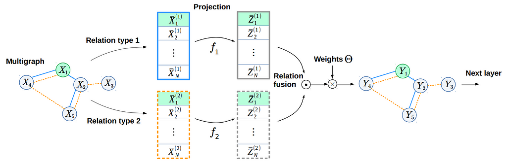
By using the proposed fusion method, implemented in the GraphLayerFusion class below, we achieve 34.5% beating the ConvNet by 1.8%, while having 2 times fewer parameters! Quite impressive for the model that initially didn’t know anything about the spatial structure of images, except for information encoded in superpixels. It would be interesting to explore other fusion methods, like this one, to get even better results.
It turned out that with a multirelational graph network and some tricks, we can do better than a Convolutional Neural Network!
Unfortunately, during our process of improving the GNN we slowly lost its invariance properties. For example, the shape of superpixels might change after rotating the image, and superpixel coordinates that we use for node features to improve the model also make it less robust.
Nevertheless, our work is a small step towards a better image reasoning model and we show that GNNs can pave a promising direction.
See my notebook on Github for implementation details.
I also highly recommend Matthias Fey’s Master’s thesis with the code on a very related topic.
Find me on Github, LinkedIn and Twitter. My homepage.
<hr><p>Can we do better than Convolutional Neural Networks? was originally published in TDS Archive on Medium, where people are continuing the conversation by highlighting and responding to this story.</p>